3 - What makes a model?

Survival analysis with tidymodels

Your turn

How do you fit a linear model in R?

How many different ways can you think of?

03:00

• lm for linear model

• glm for generalized linear model (e.g. logistic regression)

• glmnet for regularized regression

• keras for regression using TensorFlow

• stan for Bayesian regression

• spark for large data sets

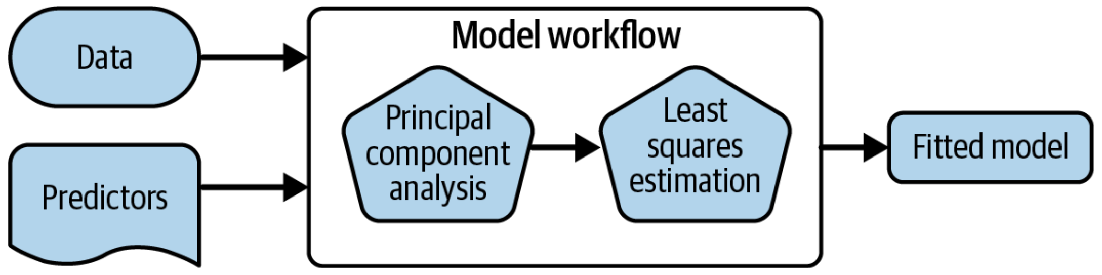
To specify a model

• Choose a model
• Specify an engine
• Set the mode

To specify a model

proportional_hazards()
#> Proportional Hazards Model Specification (censored regression)
#> 
#> Computational engine: survival

Models have default engines

To specify a model

proportional_hazards() %>%
  set_engine("glmnet")
#> Proportional Hazards Model Specification (censored regression)
#> 
#> Computational engine: glmnet

PH has only one mode, hence also a default mode

To specify a model

decision_tree()
#> Decision Tree Model Specification (unknown mode)
#> 
#> Computational engine: rpart

Some models have a default mode but not all

To specify a model

decision_tree() %>% 
  set_mode("censored regression")
#> Decision Tree Model Specification (censored regression)
#> 
#> Computational engine: rpart

All available models are listed at https://www.tidymodels.org/find/parsnip/

Your turn

Write the specification for a proportional hazards model.

Choose your engine.

All available models are listed at https://www.tidymodels.org/find/parsnip/

Extension/Challenge: Edit this code to use a different model. For example, try using a conditional inference tree as implemented in the partykit package - or try an entirely different model type!

03:00

Models we’ll be using today

• Proportional hazards (PH) model
• Decision tree

Proportional hazards model

Proportional hazards model

• Hazard modeled via a baseline hazard and a linear combination of predictors:

\(\lambda(t | x_i) = \lambda_0(t) \cdot \exp (x_i^T \beta)\)

Proportional hazards model

• Hazard modeled via a baseline hazard and a linear combination of predictors:

\(\lambda(t | x_i) = \lambda_0(t) \cdot \exp (x_i^T \beta)\)

• The hazard is proportional over all time \(t\), and thus also the probability of survival is proportional.

Decision tree

• Series of splits or if/then statements based on predictors

• First the tree grows until some condition is met (maximum depth, no more data)

• Then the tree is pruned to reduce its complexity

Decision tree

All models are wrong, but some are useful!

PH model

Decision tree

A model workflow

Workflows bind preprocessors and models

Explain that PCA that is a preprocessor / dimensionality reduction, used to decorrelate data

Fit a model spec

tree_spec <-
  decision_tree() %>% 
  set_mode("censored regression")

tree_spec %>% 
  fit(event_time ~ ., data = cat_train) 
#> parsnip model object
#> 
#> $rpart
#> n= 1765 
#> 
#> node), split, n, deviance, yval
#>       * denotes terminal node
#> 
#> 1) root 1765 1981.0090 1.0000000  
#>   2) neutered=no,unknown 696  576.4117 0.5937228 *
#>   3) neutered=yes 1069 1318.2450 1.1714650  
#>     6) intake_condition=ill_mild,ill_moderatete,normal,under_age_or_weight,other 921 1063.5830 1.0808970 *
#>     7) intake_condition=feral,fractious 148  195.7649 2.3866130 *
#> 
#> $survfit
#> 
#> Call: prodlim::prodlim(formula = form, data = data)
#> 
#> 
#> 
#> Right-censored response of a survival model
#> 
#> No.Observations: 1765 
#> 
#> Pattern:
#>                 Freq
#>  event          1116
#>  right.censored 649 
#> 
#> $levels
#> [1] "0.593722848021764" "1.08089686322063"  "2.38661313111009" 
#> 
#> attr(,"class")
#> [1] "pecRpart"

Fit a model workflow

tree_spec <-
  decision_tree() %>% 
  set_mode("censored regression")

workflow() %>%
  add_formula(event_time ~ .) %>%
  add_model(tree_spec) %>%
  fit(data = cat_train) 
#> ══ Workflow [trained] ════════════════════════════════════════════════
#> Preprocessor: Formula
#> Model: decision_tree()
#> 
#> ── Preprocessor ──────────────────────────────────────────────────────
#> event_time ~ .
#> 
#> ── Model ─────────────────────────────────────────────────────────────
#> $rpart
#> n= 1765 
#> 
#> node), split, n, deviance, yval
#>       * denotes terminal node
#> 
#> 1) root 1765 1981.0090 1.0000000  
#>   2) neutered=no,unknown 696  576.4117 0.5937228 *
#>   3) neutered=yes 1069 1318.2450 1.1714650  
#>     6) intake_condition=ill_mild,ill_moderatete,normal,under_age_or_weight,other 921 1063.5830 1.0808970 *
#>     7) intake_condition=feral,fractious 148  195.7649 2.3866130 *
#> 
#> $survfit
#> 
#> Call: prodlim::prodlim(formula = form, data = data)
#> 
#> 
#> 
#> Right-censored response of a survival model
#> 
#> No.Observations: 1765 
#> 
#> Pattern:
#>                 Freq
#>  event          1116
#>  right.censored 649 
#> 
#> $levels
#> [1] "0.593722848021763" "1.08089686322063"  "2.38661313111009" 
#> 
#> attr(,"class")
#> [1] "pecRpart"

Fit a model workflow

tree_spec <-
  decision_tree() %>% 
  set_mode("censored regression")

tree_fit <-
  workflow(event_time ~ ., tree_spec) %>% 
  fit(data = cat_train) 

Your turn

Make a workflow with your own model of choice.

Extension/Challenge: Other than formulas, what kinds of preprocessors are supported?

03:00

Predict with your model

How do you use your new tree_fit model?

predict(tree_fit, new_data = demo_cats)
#> # A tibble: 50 × 1
#>    .pred_time
#>         <dbl>
#>  1      1.08 
#>  2      0.594
#>  3      0.594
#>  4      1.08 
#>  5      2.39 
#>  6      0.594
#>  7      1.08 
#>  8      0.594
#>  9      1.08 
#> 10      0.594
#> # ℹ 40 more rows

Predict with your model

How do you use your new tree_fit model?

predict(tree_fit, new_data = demo_cats, type = "time")
#> # A tibble: 50 × 1
#>    .pred_time
#>         <dbl>
#>  1      1.08 
#>  2      0.594
#>  3      0.594
#>  4      1.08 
#>  5      2.39 
#>  6      0.594
#>  7      1.08 
#>  8      0.594
#>  9      1.08 
#> 10      0.594
#> # ℹ 40 more rows

Predict with your model

preds <- predict(tree_fit, new_data = demo_cats, type = "survival", 
                 eval_time = seq(0, 365, by = 5))
preds
#> # A tibble: 50 × 1
#>    .pred            
#>    <list>           
#>  1 <tibble [74 × 2]>
#>  2 <tibble [74 × 2]>
#>  3 <tibble [74 × 2]>
#>  4 <tibble [74 × 2]>
#>  5 <tibble [74 × 2]>
#>  6 <tibble [74 × 2]>
#>  7 <tibble [74 × 2]>
#>  8 <tibble [74 × 2]>
#>  9 <tibble [74 × 2]>
#> 10 <tibble [74 × 2]>
#> # ℹ 40 more rows

Predict with your model

preds$.pred[[1]]
#> # A tibble: 74 × 2
#>    .eval_time .pred_survival
#>         <dbl>          <dbl>
#>  1          0          1    
#>  2          5          1    
#>  3         10          0.923
#>  4         15          0.813
#>  5         20          0.749
#>  6         25          0.690
#>  7         30          0.637
#>  8         35          0.588
#>  9         40          0.536
#> 10         45          0.495
#> # ℹ 64 more rows

Predict with your model

Your turn

Run:

augment(tree_fit, new_data = demo_cats,
eval_time = seq(0, 365, by = 5))

What do you get?

03:00

The tidymodels prediction guarantee!

• The predictions will always be inside a tibble
• The column names and types are unsurprising and predictable
• The number of rows in new_data and the output are the same

The whole game - status update

Stress that fitting a model on the entire training set was only for illustrating how to fit a model