4 - Evaluating models

Survival analysis with tidymodels

An Example Model Fit

Let’s fit another PH and add some nonlinear terms via splines:

# First add all of the predictors...
f <- event_time ~ . -
  # Then remove geocoded columns
  longitude - latitude +
  # Then add them back as spline terms
  ns(longitude, df = 5) + ns(latitude, df = 5)

cat_wflow <- workflow(f, proportional_hazards())

cph_spline_fit <- cat_wflow %>%
  fit(data = cat_train)

Predictions

For our demo data set of n = 50 cats, the largest event time was 329.

We’ll make predictions from 8 days to 320 days:

demo_cat_preds <- augment(cph_spline_fit, demo_cats, eval_time = 8:320)
demo_cat_preds %>% select(1:3)
#> # A tibble: 50 × 3
#>    .pred              .pred_time event_time
#>    <list>                  <dbl>     <Surv>
#>  1 <tibble [313 × 5]>       58.9        36 
#>  2 <tibble [313 × 5]>      181.         16+
#>  3 <tibble [313 × 5]>      106.         12+
#>  4 <tibble [313 × 5]>       62.7        16 
#>  5 <tibble [313 × 5]>       31.4        22 
#>  6 <tibble [313 × 5]>       88.5        16 
#>  7 <tibble [313 × 5]>       48.2       294 
#>  8 <tibble [313 × 5]>      109.         68+
#>  9 <tibble [313 × 5]>       60.9        31 
#> 10 <tibble [313 × 5]>      104.         24+
#> # ℹ 40 more rows

Concordance

The concordance statistic (“c-index”, Harrell et al (1996)) is a metric that quantifies that the rank order of the times is consistent with some model score (e.g., a survival probability).

It takes into account censoring and does not depend on a specific evaluation time. The range of values is \([-1, 1]\).

demo_cat_preds %>% 
  concordance_survival(event_time, estimate = .pred_time)
#> # A tibble: 1 × 3
#>   .metric              .estimator .estimate
#>   <chr>                <chr>          <dbl>
#> 1 concordance_survival standard       0.668

Time-dependent metrics

We pick specific time points to evaluate the model (depending on our problem) such as every 30 days:

Classification(ish) Metrics

Most dynamic metrics convert the survival probabilities to events and non-events based on some probability threshold.

From there, we can apply existing classification metrics, such as

• Brier Score (for calibration)
• Area under the ROC curve (for separation)

We’ll talk about both of these.

There are more details on dynamics metrics at tidymodels.org.

Converting to Events

For a specific evaluation time point \(\tau\), we convert the observed event time to a binary event/non-event version (if possible) (\(y_{i\tau} \in \{0, 1\}\)).

\[ y_{i\tau} = \begin{cases} 1 & \text{if } t_{i} \leq \tau\text{ and event} \notag \\ 0 & \text{if } t_{i} \gt \tau \text{ and } either \notag \\ missing & \text{if } t_{i} \leq \tau\text{ and censored } \end{cases} \]

Converting to Events

Dealing with Missing Outcome Data

Without censored data points, this conversion would yield appropriate performance estimates since no event outcomes would be missing.

Otherwise, there is the potential for bias due to missingness.

We’ll use tools from causal inference to compensate by creating a propensity score that uses the probability of being censored/missing.

Case weights use the inverse of this probability. See Graf et al (1999).

Brier Score

The Brier score is calibration metric originally meant for classification models:

\[ Brier = \frac{1}{N}\sum_{i=1}^N\sum_{k=1}^C (y_{ik} - \hat{\pi}_{ik})^2 \]

For our application, we have two classes and case weights

\[ Brier(t) = \frac{1}{W}\sum_{i=1}^N w_{it}\left[\underbrace{I(y_{it} = 0)(y_{it} - \hat{p}_{it})^2}_\text{non-events} + \underbrace{I(y_{it} = 1)(y_{it} - (1 - \hat{p}_{it}))^2}_\text{events}\right] \]

Brier Scores

demo_brier <- brier_survival(demo_cat_preds, truth = event_time, .pred)
demo_brier %>% filter(.eval_time %in% seq(30, 300, by = 30))
#> # A tibble: 10 × 4
#>    .metric        .estimator .eval_time .estimate
#>    <chr>          <chr>           <dbl>     <dbl>
#>  1 brier_survival standard           30     0.163
#>  2 brier_survival standard           60     0.170
#>  3 brier_survival standard           90     0.151
#>  4 brier_survival standard          120     0.174
#>  5 brier_survival standard          150     0.164
#>  6 brier_survival standard          180     0.188
#>  7 brier_survival standard          210     0.147
#>  8 brier_survival standard          240     0.156
#>  9 brier_survival standard          270     0.161
#> 10 brier_survival standard          300     0.125

Brier Scores Over Evaluation Time

Integrated Brier Score

brier_survival_integrated(demo_cat_preds, truth = event_time, .pred)
#> # A tibble: 1 × 3
#>   .metric                   .estimator .estimate
#>   <chr>                     <chr>          <dbl>
#> 1 brier_survival_integrated standard       0.152

Area Under the ROC Curve

This is more straightforward.

We can use the standard ROC curve machinery once we have the indicators, probabilities, and censoring weights at evaluation time \(\tau\) (Hung and Chiang (2010)).

ROC curves measure the separation between events and non-events and are ignorant of how well-calibrated the probabilities are.

Area Under the ROC Curve

demo_roc_auc <- roc_auc_survival(demo_cat_preds, truth = event_time, .pred)
demo_roc_auc %>% filter(.eval_time %in% seq(30, 300, by = 30))
#> # A tibble: 10 × 4
#>    .metric          .estimator .eval_time .estimate
#>    <chr>            <chr>           <dbl>     <dbl>
#>  1 roc_auc_survival standard           30     0.660
#>  2 roc_auc_survival standard           60     0.679
#>  3 roc_auc_survival standard           90     0.582
#>  4 roc_auc_survival standard          120     0.582
#>  5 roc_auc_survival standard          150     0.515
#>  6 roc_auc_survival standard          180     0.515
#>  7 roc_auc_survival standard          210     0.490
#>  8 roc_auc_survival standard          240     0.490
#>  9 roc_auc_survival standard          270     0.490
#> 10 roc_auc_survival standard          300     0.679

ROC AUC Over Evaluation Time

Using Evaluation Times

When predicting, you can get predictions at any values of \(\tau\).

During model development, we suggest picking a more focused set of evaluation times (for computational time).

You should also pick a time to perform your optimizations/comparisons and list that value first in the vector. If 90 days was of interest, you might use

times <- c(90, 30, 60, 120)

⚠️ DANGERS OF OVERFITTING ⚠️

Your turn

Why haven’t we done this?

cph_spline_fit %>%
  augment(cat_train, eval_time = 8:320) %>%
  brier_survival(truth = event_time, .pred)

05:00

• repredicting the training set is overly optimistic
• optimising that leads to overfitting

The testing data are precious 💎

How can we use the training data to compare and evaluate different models? 🤔

Cross-validation

set.seed(123)
cat_folds <- vfold_cv(cat_train, v = 10)# v = 10 is default
cat_folds
#> #  10-fold cross-validation 
#> # A tibble: 10 × 2
#>    splits             id    
#>    <list>             <chr> 
#>  1 <split [1588/177]> Fold01
#>  2 <split [1588/177]> Fold02
#>  3 <split [1588/177]> Fold03
#>  4 <split [1588/177]> Fold04
#>  5 <split [1588/177]> Fold05
#>  6 <split [1589/176]> Fold06
#>  7 <split [1589/176]> Fold07
#>  8 <split [1589/176]> Fold08
#>  9 <split [1589/176]> Fold09
#> 10 <split [1589/176]> Fold10

Cross-validation

What is in this?

cat_folds <- vfold_cv(cat_train)
cat_folds$splits[1:3]
#> [[1]]
#> <Analysis/Assess/Total>
#> <1588/177/1765>
#> 
#> [[2]]
#> <Analysis/Assess/Total>
#> <1588/177/1765>
#> 
#> [[3]]
#> <Analysis/Assess/Total>
#> <1588/177/1765>

Set the seed when creating resamples

Talk about a list column, storing non-atomic types in dataframe

Bootstrapping

set.seed(3214)
bootstraps(cat_train)
#> # Bootstrap sampling 
#> # A tibble: 25 × 2
#>    splits             id         
#>    <list>             <chr>      
#>  1 <split [1765/657]> Bootstrap01
#>  2 <split [1765/644]> Bootstrap02
#>  3 <split [1765/625]> Bootstrap03
#>  4 <split [1765/638]> Bootstrap04
#>  5 <split [1765/647]> Bootstrap05
#>  6 <split [1765/655]> Bootstrap06
#>  7 <split [1765/655]> Bootstrap07
#>  8 <split [1765/637]> Bootstrap08
#>  9 <split [1765/669]> Bootstrap09
#> 10 <split [1765/638]> Bootstrap10
#> # ℹ 15 more rows

The whole game - status update

We are equipped with metrics and resamples!

Fit our model to the resamples

cat_res <- fit_resamples(cat_wflow, cat_folds, eval_time = c(90, 30, 60, 120))
cat_res
#> # Resampling results
#> # 10-fold cross-validation 
#> # A tibble: 10 × 4
#>    splits             id     .metrics         .notes          
#>    <list>             <chr>  <list>           <list>          
#>  1 <split [1588/177]> Fold01 <tibble [4 × 5]> <tibble [0 × 3]>
#>  2 <split [1588/177]> Fold02 <tibble [4 × 5]> <tibble [0 × 3]>
#>  3 <split [1588/177]> Fold03 <tibble [4 × 5]> <tibble [0 × 3]>
#>  4 <split [1588/177]> Fold04 <tibble [4 × 5]> <tibble [0 × 3]>
#>  5 <split [1588/177]> Fold05 <tibble [4 × 5]> <tibble [0 × 3]>
#>  6 <split [1589/176]> Fold06 <tibble [4 × 5]> <tibble [0 × 3]>
#>  7 <split [1589/176]> Fold07 <tibble [4 × 5]> <tibble [0 × 3]>
#>  8 <split [1589/176]> Fold08 <tibble [4 × 5]> <tibble [0 × 3]>
#>  9 <split [1589/176]> Fold09 <tibble [4 × 5]> <tibble [0 × 3]>
#> 10 <split [1589/176]> Fold10 <tibble [4 × 5]> <tibble [0 × 3]>

Evaluating model performance

cat_res %>%
  collect_metrics()
#> # A tibble: 4 × 7
#>   .metric        .estimator .eval_time  mean     n std_err .config             
#>   <chr>          <chr>           <dbl> <dbl> <int>   <dbl> <chr>               
#> 1 brier_survival standard           30 0.212    10 0.00413 Preprocessor1_Model1
#> 2 brier_survival standard           60 0.246    10 0.00555 Preprocessor1_Model1
#> 3 brier_survival standard           90 0.207    10 0.00677 Preprocessor1_Model1
#> 4 brier_survival standard          120 0.158    10 0.0105  Preprocessor1_Model1

collect_metrics() is one of a suite of collect_*() functions that can be used to work with columns of tuning results. Most columns in a tuning result prefixed with . have a corresponding collect_*() function with options for common summaries.

We can reliably measure performance using only the training data 🎉

Where are the fitted models?

cat_res
#> # Resampling results
#> # 10-fold cross-validation 
#> # A tibble: 10 × 4
#>    splits             id     .metrics         .notes          
#>    <list>             <chr>  <list>           <list>          
#>  1 <split [1588/177]> Fold01 <tibble [4 × 5]> <tibble [0 × 3]>
#>  2 <split [1588/177]> Fold02 <tibble [4 × 5]> <tibble [0 × 3]>
#>  3 <split [1588/177]> Fold03 <tibble [4 × 5]> <tibble [0 × 3]>
#>  4 <split [1588/177]> Fold04 <tibble [4 × 5]> <tibble [0 × 3]>
#>  5 <split [1588/177]> Fold05 <tibble [4 × 5]> <tibble [0 × 3]>
#>  6 <split [1589/176]> Fold06 <tibble [4 × 5]> <tibble [0 × 3]>
#>  7 <split [1589/176]> Fold07 <tibble [4 × 5]> <tibble [0 × 3]>
#>  8 <split [1589/176]> Fold08 <tibble [4 × 5]> <tibble [0 × 3]>
#>  9 <split [1589/176]> Fold09 <tibble [4 × 5]> <tibble [0 × 3]>
#> 10 <split [1589/176]> Fold10 <tibble [4 × 5]> <tibble [0 × 3]>

🗑️

But it’s easy to save the predictions

# Save the assessment set results
ctrl_cat <- control_resamples(save_pred = TRUE)
cat_res <- fit_resamples(cat_wflow, cat_folds, eval_time = c(90, 30, 60, 120),
                         control = ctrl_cat)

cat_res
#> # Resampling results
#> # 10-fold cross-validation 
#> # A tibble: 10 × 5
#>    splits             id     .metrics         .notes           .predictions
#>    <list>             <chr>  <list>           <list>           <list>      
#>  1 <split [1588/177]> Fold01 <tibble [4 × 5]> <tibble [0 × 3]> <tibble>    
#>  2 <split [1588/177]> Fold02 <tibble [4 × 5]> <tibble [0 × 3]> <tibble>    
#>  3 <split [1588/177]> Fold03 <tibble [4 × 5]> <tibble [0 × 3]> <tibble>    
#>  4 <split [1588/177]> Fold04 <tibble [4 × 5]> <tibble [0 × 3]> <tibble>    
#>  5 <split [1588/177]> Fold05 <tibble [4 × 5]> <tibble [0 × 3]> <tibble>    
#>  6 <split [1589/176]> Fold06 <tibble [4 × 5]> <tibble [0 × 3]> <tibble>    
#>  7 <split [1589/176]> Fold07 <tibble [4 × 5]> <tibble [0 × 3]> <tibble>    
#>  8 <split [1589/176]> Fold08 <tibble [4 × 5]> <tibble [0 × 3]> <tibble>    
#>  9 <split [1589/176]> Fold09 <tibble [4 × 5]> <tibble [0 × 3]> <tibble>    
#> 10 <split [1589/176]> Fold10 <tibble [4 × 5]> <tibble [0 × 3]> <tibble>

But it’s easy to collect the predictions

cat_preds <- collect_predictions(cat_res)
cat_preds
#> # A tibble: 1,765 × 5
#>    .pred            id      .row event_time .config             
#>    <list>           <chr>  <int>     <Surv> <chr>               
#>  1 <tibble [4 × 3]> Fold01    13       139  Preprocessor1_Model1
#>  2 <tibble [4 × 3]> Fold01    14        40  Preprocessor1_Model1
#>  3 <tibble [4 × 3]> Fold01    33        10+ Preprocessor1_Model1
#>  4 <tibble [4 × 3]> Fold01    52       121  Preprocessor1_Model1
#>  5 <tibble [4 × 3]> Fold01    55        39+ Preprocessor1_Model1
#>  6 <tibble [4 × 3]> Fold01    70        15+ Preprocessor1_Model1
#>  7 <tibble [4 × 3]> Fold01    84        35  Preprocessor1_Model1
#>  8 <tibble [4 × 3]> Fold01    91        18  Preprocessor1_Model1
#>  9 <tibble [4 × 3]> Fold01    93        82+ Preprocessor1_Model1
#> 10 <tibble [4 × 3]> Fold01   100        11+ Preprocessor1_Model1
#> # ℹ 1,755 more rows

Decision tree 🌳

Random forest 🌳🌲🌴🌵🌴🌳🌳🌴🌲🌵🌴🌲🌳🌴🌳🌵🌵🌴🌲🌲🌳🌴🌳🌴🌲🌴🌵🌴🌲🌴🌵🌲🌵🌴🌲🌳🌴🌵🌳🌴🌳

Random forest 🌳🌲🌴🌵🌳🌳🌴🌲🌵🌴🌳🌵

• Ensemble many decision tree models

• All the trees vote! 🗳️

• Bootstrap aggregating + random predictor sampling

• Often works well without tuning hyperparameters (more on this in a moment), as long as there are enough trees

Create a random forest model

rf_spec <- rand_forest(trees = 1000) %>% 
  set_engine("aorsf") %>% 
  set_mode("censored regression")
rf_spec
#> Random Forest Model Specification (censored regression)
#> 
#> Main Arguments:
#>   trees = 1000
#> 
#> Computational engine: aorsf

Create a random forest model

rf_wflow <- workflow(event_time ~ ., rf_spec)
rf_wflow
#> ══ Workflow ══════════════════════════════════════════════════════════
#> Preprocessor: Formula
#> Model: rand_forest()
#> 
#> ── Preprocessor ──────────────────────────────────────────────────────
#> event_time ~ .
#> 
#> ── Model ─────────────────────────────────────────────────────────────
#> Random Forest Model Specification (censored regression)
#> 
#> Main Arguments:
#>   trees = 1000
#> 
#> Computational engine: aorsf

Your turn

Use fit_resamples() and rf_wflow to:

• keep predictions
• compute metrics

08:00

Evaluating model performance

ctrl_cat <- control_resamples(save_pred = TRUE)

# Random forest uses random numbers so set the seed first
set.seed(2)
rf_res <- fit_resamples(rf_wflow, cat_folds, eval_time = c(90, 30, 60, 120), 
                        control = ctrl_cat)

collect_metrics(rf_res)
#> # A tibble: 4 × 7
#>   .metric        .estimator .eval_time  mean     n std_err .config             
#>   <chr>          <chr>           <dbl> <dbl> <int>   <dbl> <chr>               
#> 1 brier_survival standard           30 0.210    10 0.00423 Preprocessor1_Model1
#> 2 brier_survival standard           60 0.243    10 0.00520 Preprocessor1_Model1
#> 3 brier_survival standard           90 0.200    10 0.00731 Preprocessor1_Model1
#> 4 brier_survival standard          120 0.151    10 0.0103  Preprocessor1_Model1

The whole game - status update

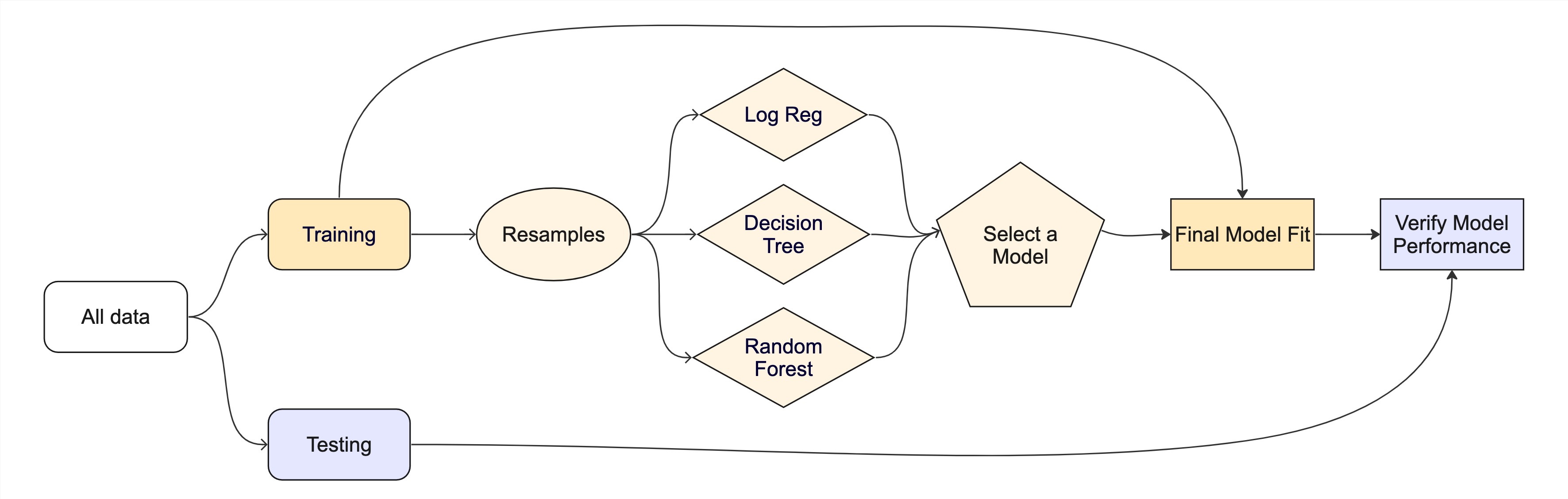
The final fit

Suppose that we are happy with our random forest model.

Let’s fit the model on the training set and verify our performance using the test set.

We’ve shown you fit() and predict() (+ augment()) but there is a shortcut:

# cat_split has train + test info
final_fit <- last_fit(rf_wflow, cat_split, eval_time = c(90, 30, 60, 120)) 

final_fit
#> # Resampling results
#> # Manual resampling 
#> # A tibble: 1 × 6
#>   splits             id               .metrics .notes   .predictions .workflow 
#>   <list>             <chr>            <list>   <list>   <list>       <list>    
#> 1 <split [1765/442]> train/test split <tibble> <tibble> <tibble>     <workflow>

What is in final_fit?

collect_metrics(final_fit)
#> # A tibble: 4 × 5
#>   .metric        .estimator .eval_time .estimate .config             
#>   <chr>          <chr>           <dbl>     <dbl> <chr>               
#> 1 brier_survival standard           30     0.217 Preprocessor1_Model1
#> 2 brier_survival standard           60     0.225 Preprocessor1_Model1
#> 3 brier_survival standard           90     0.160 Preprocessor1_Model1
#> 4 brier_survival standard          120     0.108 Preprocessor1_Model1

These are metrics computed with the test set

What is in final_fit?

extract_workflow(final_fit)
#> ══ Workflow [trained] ════════════════════════════════════════════════
#> Preprocessor: Formula
#> Model: rand_forest()
#> 
#> ── Preprocessor ──────────────────────────────────────────────────────
#> event_time ~ .
#> 
#> ── Model ─────────────────────────────────────────────────────────────
#> ---------- Oblique random survival forest
#> 
#>      Linear combinations: Accelerated Cox regression
#>           N observations: 1765
#>                 N events: 1116
#>                  N trees: 1000
#>       N predictors total: 18
#>    N predictors per node: 6
#>  Average leaves per tree: 142.739
#> Min observations in leaf: 5
#>       Min events in leaf: 1
#>           OOB stat value: 0.63
#>            OOB stat type: Harrell's C-index
#>      Variable importance: anova
#> 
#> -----------------------------------------

Use this for prediction on new data, like for deploying

The whole game